Transfer Learning in Computer Vision
Recall when beginning to train a neural network its weights might be initialized randomly. What if you could start training with a leg up because the network already has some useful information inside of it? Transfer learning is that leg up where you can repurpose models trained on similar tasks and use them for your specific task instead of training from scratch.
Benefits include:
- training faster
- less training data
- boosts generalization
- might improve accuracy
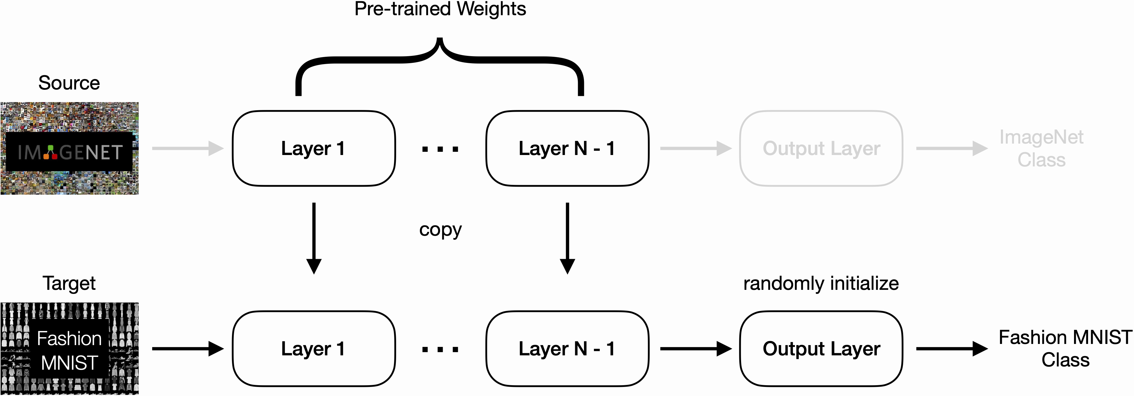
Above we see an example of using ImageNet pre-trained weights to classify objects from the Fashion MNIST dataset. A bit of an overkill example, but you get the point.
There are three main ways you might go about transfer learning:
-
Use the pre-trained model as a pre-trained feature extractor by freezing its hidden layers (and replacing its head with your own). This works well when your task isn’t too different from the pre-trained model’s task.
-
Finetune the pre-trained model completely by not freezing any layers
-
Finetune but freeze some number layers. There are two main risks with this approach: (1) the higher-level early neurons are more specialized than we expected, and (2) splitting & combining two arbitrary layers causes a mismatch in learned features that cannot be relearned by earlier layers.
Thanks to the open-source community there are many places you can find pre-trained models, like PyTorch Hub, HuggingFace, and TensorFlow Hub to name a few.
Segmentation Example
1. Loading the Model
I’ve used the DeepLabv3 model from Pytorch Hub and gotten some pretty great results. We first start by loading the pre-trained weights into the model:
import torchvision

# there are three model sizes: MobileNet, ResNet50, and ResNet101
weights = torchvision.models.segmentation.DeepLabV3_ResNet50_Weights.DEFAULT
model = torchvision.models.segmentation.deeplabv3_resnet50(weights=weights).to(device)
Then we need to replace the classifier layer but to do that we need to know its input dimension. The easiest way I’ve found to do that is to use torchinfo.summary():
from torchinfo import summary

summary(
    model=model,
    input_size=(2, 3, 1024, 1024),
    col_names=["input_size", "output_size", "num_params", "trainable"],
    col_width=20,
    row_settings=["var_names"]
)
which prints out:
===========================================================================================================================
Layer (type (var_name))                            Input Shape          Output Shape         Param #              Trainable
===========================================================================================================================
DeepLabV3 (DeepLabV3)                              [2, 3, 1024, 1024]   [2, 2, 1024, 1024]   --                   True
├─IntermediateLayerGetter (backbone)               [2, 3, 1024, 1024]   [2, 2048, 128, 128]  --                   True
│    └─Conv2d (conv1)                              [2, 3, 1024, 1024]   [2, 64, 512, 512]    9,408                True
│    └─BatchNorm2d (bn1)                           [2, 64, 512, 512]    [2, 64, 512, 512]    128                  True
│    └─ReLU (relu)                                 [2, 64, 512, 512]    [2, 64, 512, 512]    --                   --
│    └─MaxPool2d (maxpool)                         [2, 64, 512, 512]    [2, 64, 256, 256]    --                   --
│    └─Sequential (layer1)                         [2, 64, 256, 256]    [2, 256, 256, 256]   --                   True
│    │    └─Bottleneck (0)                         [2, 64, 256, 256]    [2, 256, 256, 256]   75,008               True
│    │    └─Bottleneck (1)                         [2, 256, 256, 256]   [2, 256, 256, 256]   70,400               True
│    │    └─Bottleneck (2)                         [2, 256, 256, 256]   [2, 256, 256, 256]   70,400               True
.                                                           .                                                       .
.                                                           .                                                       .
.                                                           .                                                       .
├─DeepLabHead (classifier)                         [2, 2048, 128, 128]  [2, 2, 128, 128]     --                   True
│    └─ASPP (0)                                    [2, 2048, 128, 128]  [2, 256, 128, 128]   --                   True
│    │    └─ModuleList (convs)                     --                   --                   15,206,912           True
│    │    └─Sequential (project)                   [2, 1280, 128, 128]  [2, 256, 128, 128]   328,192              True
│    └─Conv2d (1)                                  [2, 256, 128, 128]   [2, 256, 128, 128]   589,824              True
│    └─BatchNorm2d (2)                             [2, 256, 128, 128]   [2, 256, 128, 128]   512                  True
│    └─ReLU (3)                                    [2, 256, 128, 128]   [2, 256, 128, 128]   --                   --
│    └─Conv2d (4)                                  [2, 256, 128, 128]   [2, 2, 128, 128]     514                  True
===========================================================================================================================
Total params: 39,633,986
Trainable params: 39,633,986
Non-trainable params: 0
Total mult-adds (T): 1.31
===========================================================================================================================
Input size (MB): 25.17
Forward/backward pass size (MB): 17650.16
Params size (MB): 158.54
Estimated Total Size (MB): 17833.87
===========================================================================================================================
From the DeepLabHead (classifier) line which has shape [batch, in_channels, height, width] we can see that we need in_channels=2048 for our new classifier.
# modify classifier layer for desired number of classes
# number for in_channels was found by examining the model architecture
model.classifier = DeepLabHead(in_channels=2048, num_classes=NUM_CLASSES)
2. Tensor Shapes
Then let’s try and understand the model’s output. From its documentation: “The model returns an OrderedDict with two Tensors that are of the same height and width as the input Tensor … output['out'] contains the semantic masks, and output['aux'] contains the auxiliary loss values per-pixel.”
# output['out'] is what we really want
# output is a tensor with shape [batch_size, num_classes, height, width]
output = model(X_train.to(device))["out"]
In order to calculate the loss we have to massage the tensors a bit. I chose nn.CrossEntropyLoss() as the loss function and its documentation allows the input to have shape [batch_size, num_classes, height, width] but its target must have shape [batch_size, height, width] so with help from the einops package:
from einops import rearrange

# rearrange target
target = rearrange(target, "bat cla height width -> (bat cla) height width")

# calculate loss
loss = loss_fn(output, target)
Now we notice that for each batch there is a dimension in the first index of the tensor for logit(false) and logit(true) which is redundant. We can just keep logit(true) for each batch, take that softmax, binarize the predictions, and finally calculate accuracy.
# modify output to be in format [logit(true)] for each sample
output = output[:, 1, :, :]

# take softmax
output = nn.functional.softmax(output, dim=1)

# binarize predictions & calculate accuracy
y_pred = (output > 0.5).type(torch.int32)
accuracy_fn = torchmetrics.Accuracy(task="binary", num_classes=NUM_CLASSES)
accuracy = accuracy_fn(y_pred)
3. Wrapping Up
With the loss and accuracy for a batch we can go ahead and train our model. The only other trouble I had with with my custom dataset was that I didn’t realize torchvision.transforms.ToTensor() automatically divides a tensor by 256 so make sure your data is correctly scaled!
For experiment tracking I used wandb which was super simple to set up and let me easily visualize how tweaking some hyperparameters like batch size affected this model’s training. You can find how I created the dataset class, training loops, and experiment tracking for segmentation transfer learning in my GitHub repository.
Classification Example
Transfer learning for a classification task is virtually the same as segmentation and slightly easier. We start again by loading the pre-trained weights into the model and replacing the classifier layer so that it has the right input and output dimensions for our target problem.
import torchvision

# there are multiple other model sizes
weights = torchvision.models.EfficientNet_B0_Weights.DEFAULT
model = torchvision.models.efficientnet_b0(weights=weights).to(device)

# if you wanted to freeze base layers
for param in model.features.parameters():
    param.requires_grad = False

# modify classifier layer for number of classes
# added dropout for more robustness
model.classifier = nn.Sequential(
    torch.nn.Dropout(p=0.2, inplace=True),
    nn.Linear(in_features=CLASSIFIER_IN_FEATURES, out_features=NUM_CLASSES),
).to(device)
The only tricky thing here is calculating CLASSIFIER_IN_FEATURES, which was found by printing out the model’s layers using torchinfo.summary(). The training step is more straightforward than the segmentation example:
# forward pass
# outputs are in the format [logit(true)] for each sample
# logit = log(unnormalized probability)
outputs = model(X_train.to(device))

# calculate loss & accuracy
loss = loss_fn(outputs, y_train)
accuracy = accuracy_fn(outputs, y_train)
There you have it, now you can use transfer learning for both segmentation and classification tasks.