Physics-Constrained Neural Networks for Solving Partial Differential Equations
Background
A neural network learns a function to map inputs to outputs. Because solutions to differential equations are also functions we can use neural networks to solve them!
Oftentimes in physics we want solutions to differential equations that obey the laws of physics. For example, we don’t want solutions that violate conservation laws or predict things like negative mass or density. How do we force a neural network to only predict functions that satisfy some physical constraint?
Darcy Flow
Let’s take the example of 2D darcy flow, a time-independent partial differential equation (PDE) that describes the flow of a fluid through a porous medium. The solution to this PDE tells us the pressure distribution of the fluid at a given spatial point - and from that we can derive the flow rate and direction of fluid motion.
Darcy flow states:
\[\begin{align} -\nabla \cdot q &= f(x,y) && x,y \in (0,1) \tag{1} \newline q &= \nu(x,y) \nabla u(x,y) && \tag{2} \newline \end{align}\]With boundary condition
\[\begin{align} \underbrace{u(x,y)}_{\text{PDE solution}} &= 0 && \qquad \qquad \quad x,y \in \partial(0,1)^2 \tag{3} \end{align}\]Where: \begin{align} u(x, y) &= \text{pressure distribution}, \newline q &= \text{flow rate}, \newline \nu(x, y) &= \text{diffusion coefficient}, \newline \nabla &= \text{divergence operator}, \newline f(x, y) &= \begin{cases} \text{source} & \text{if } f(x, y) > 0 \newline \text{sink} & \text{if } f(x, y) < 0 \end{cases} = 1 \end{align}
We can boil this fancy law down to a conservation of mass. In english, eq. \((1)\) states that the amount of fluid entering a region (\(-\nabla \cdot q\)) must either leave it or be accounted for by the source / sink (\(f(x,y)\)). For this problem, we’re setting \(f(x,y) = 1\) as a hard constraint to mean that there is a constant source of fluid in the system and we want to learn a model that predicts the pressure distribution. We’re going to train a model to solve the PDE given the hard, physics, constraint.
Data
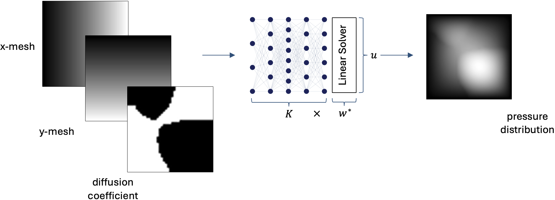
The dataset we’re using gives us the diffusion coefficient \(\nu(x, y)\) as input and has the pressure distribution \(u(x,y)\) as output labels. The model is then learning the relationship of how different materials’ diffusion coefficients affect how fluids flow through them. In order to discretize the problem we’re also going to pass in a finite mesh so that our model has a spatial box to operate on. The mesh grid stays the same for every sample, but the diffusion coefficient changes. So the shapes of these are:
- Mesh: [Batch, \(N_x\), \(N_y\), 2] where \(N_x\) & \(N_y\) are the number of grid points and 2 represents the x,y coordinates at each point
- Diffusion coefficient \(\nu\): [Batch, \(N_x\), \(N_y\), 1] the same as above except we only have 1 dimension to predict for each grid point
Data is available courtesy of the Anima AI + Science Lab Lab at CalTech as part of their work [3]. For training data we will use the url [4] and for validation the url [5].
Constrained Model
Ok great, we have a partial differential equation and our goal is to train a neural network that guesses solutions to this. In our heads, we imagine our solutions could be expressed as a linear combination of basis functions and their corresponding weights. This is a fancy way of saying that our final function might be comprised of applying combinations of differently sized lego-brick functions.
\[u = \sum_i K_i w_i \tag{4}\]Where:
\begin{align}
K &= \text{set of basis functions}, \\
w &= \text{weights for each basis function} \\
\end{align}
Now we see a problem - we need to optimize two things with this approach: generating optimal basis functions in addition to optimal weights for our final prediction to be good. This type of problem is called bi-level optimization and we’re gonna solve it with wizardry (or at least I think so).
So now our plan is to have the neural network predict the basis functions, and then we’ll stack a linear solver to calculate the weights. The solver will ensure they satisfy the constraint imposed by the forcing function \(f(x,y)=1\). In other words, the linear solver layer is how we implement our physical constraint.
\begin{align} K(\theta) w^{\ast}(\theta) = f(x,y) \iff K(\theta) w^{\ast}(\theta) - 1 = 0 & \tag{5} \newline \end{align}
(using \(w^*\) to represent the optimal weights for a given set of basis functions \(K\)).
How to Backpropagate?
In order for our model to learn anything we’re going to need to pass the gradients backwards from the linear solver layer to the ResNet. In an ideal world we could simply write out a chain rule like so:
\[\frac{\partial \mathcal{L}}{\partial \theta} = \frac{\partial \mathcal{L}}{\partial w^{*}} \cdot \frac{\partial w^{*}}{\partial \theta} \tag{6}\]But with this weird linear solver layer in our system what is the relationship between between its weights and the neural network’s weights? Is it computationally feasible to directly calculate \(\frac{\partial \mathcal{L}}{\partial w^{*}}\)? To do so would mean we would have to find the gradients of each step of the solver with respect to the parameters, for every iteration it takes to converge. This quickly becomes a nightmare in terms of computation, memory, and stability.
Instead of doing that we could also link \(w^*(\theta)\) and \(\theta\) through the optimality condition we defined in eq. \((5)\). However, because the linear solver’s weights \(w\) don’t have an explicit dependence on \(\theta\), we’ll have to differentiate the expression implicitly [1]:
\[\begin{align} \frac{\partial}{\partial \theta} \left( K(\theta) w^{\ast}(\theta) - 1 \right) = 0 \newline \underbrace{\frac{\partial F}{\partial w}}_{A} \underbrace{\frac{\partial w^*(\theta)}{\partial \theta}}_{J_1} + \underbrace{\frac{\partial F}{\partial K}}_{B} \frac{\partial K(\theta)}{\partial \theta} = 0 & \tag{7} \newline \end{align}\]We can directly compute \(A\) and \(B\) as outputs of the forward pass and our weights:
\[\begin{align} A &= \frac{\partial}{\partial w} \left( K(\theta) w - 1 \right) = K(\theta), \newline B &= \frac{\partial}{\partial K} \left( K w(\theta) - 1 \right) = w^*(\theta), \newline J_1 &= \frac{\partial w^*(\theta)}{\partial \theta} = \quad ? \end{align}\]But what is \(J_1\)? Let’s rearrange our expression to see if we can solve for it.
\[\begin{align} AJ_1 + B \frac{\partial K(\theta)}{\partial \theta} = 0 \newline J_1 = A^{-1} B \frac{\partial K(\theta)}{\partial \theta} \newline \frac{\partial w^*(\theta)}{\partial \theta} = -K(\theta)^{-1} w^*(\theta) \frac{\partial K}{\partial \theta} \tag{8} \end{align}\]Great! So now we can compute all the terms that lead to \(\frac{\partial w^*}{\partial \theta}\). Let’s substitute our expression in eq. \((8)\) into eq. \((6)\):
\[\frac{\partial \mathcal{L}}{\partial \theta} = - \frac{\partial \mathcal{L}}{\partial w^{*}} \cdot K(\theta)^{-1} w^*(\theta) \frac{\partial K}{\partial \theta} \tag{9}\]We now have a way to backpropagate through the linear solver 🎉
Implementation
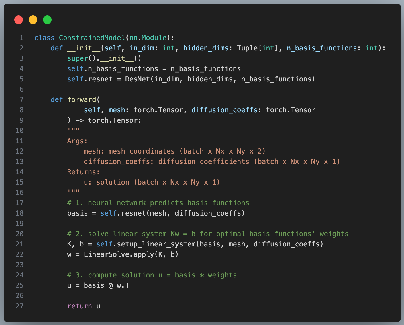
Our model class is going to look something like this:
But in order to pass gradients through the LinearSolve layer we’re going to have to tell PyTorch our new backward pass rule:
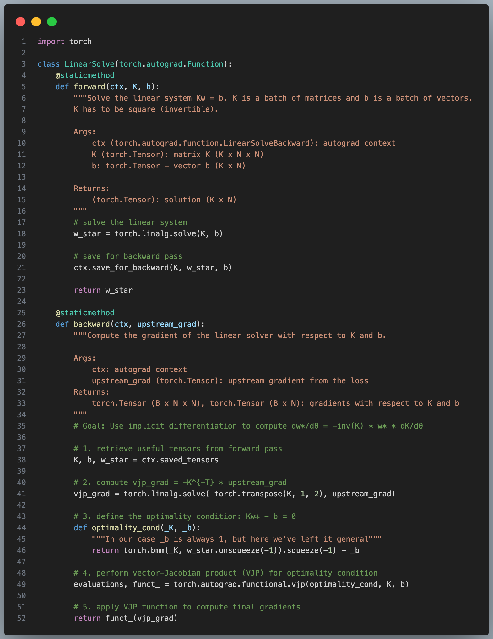
Ok so there’s a lot going on here so let’s break it down. For the implementation we rewrite eq. \((9)\) like so:
\[\frac{\partial \mathcal{L}}{\partial \theta} = w^*(\theta) \cdot \underbrace{v \cdot -K(\theta)^{-1}}_{\texttt{vjp_grad}} \underbrace{\frac{\partial K}{\partial \theta}}_{J_2} \tag{10}\]Where
\[\begin{align} v &= \frac{\partial \mathcal{L}}{\partial w^{*}} = \text{upstream gradient}, \newline J_2 &= \text{Jacobian of the function $K$ with respect to $\theta$} \newline \end{align}\]\(\texttt{vjp_grad} \times J_2\) is called a vector-Jacobian product (VJP) and it’s the reason why reverse-mode auto differentiation is so efficient [6]. Because taking the inverse of a matrix in \(K^{-1}\) is sometimes not numerically stable we instead find \(\texttt{vjp_grad}\) by solving the linear system:
\[\begin{align} K^Tx = - \frac{\partial \mathcal{L}}{\partial w^{*}} \tag{11} \newline \end{align}\]Then we formulate a functional form of the VJP and finally apply it to vjp_grad.
References:
- [1] Efficient and Modular Implicit Differentiation
- [2] Learning Differentiable Solvers For Systems With Hard Constraints
- [3] Fourier Neural Operator for Parametric Partial Differential Equations
- [4] Darcy Flow Training Data
- [5] Darcy Flow Validation Data
- [6] To jog the memory, the Jacobian is the matrix of all partial derivatives for a function.
But if we have a large neural network calculating the entire Jacobian matrix becomes too computationally expensive. Instead we take advantage of its structure by only multiplying the upstream grad \(v\) with every row of \(J\) without ever having to instantiate \(J\) in its entirety.